Overview
Python modules
The backend for the NIRWALS Simulator is implemented as a Django application. The code for carrying out the simulations (as explained on the simulator physics page) is found in four modules:
nirwals.physics.bandpass-
Functions for throughput calculations. (View documentation.)
nirwals.physics.exposure-
Functions for signal-to-noise ratio calculations. (View documentation.)
nirwals.physics.spectrum-
Functions for generating the source and sky background spectra. (View documentation.)
nirwals.physics.utils-
Utility functions. (View documentation.)
If you are interested in the code for implementing the URL routes etc., you may have a look at the project repository.
Implementation notes
Below are some implementation notes. We use synphot for implementing the backend, and unless stated otherwise class and method names refer to this library.
Spectra
All spectra are realised as SourceSpectrum instances. Where applicable, a normalised spectrum is generated with a custom normalize method. synphot's Johnson J bandpass is used for normalisation.
Blackbody
The BlackBodyNorm1D model is used with the user-supplied temperature and redshift. The resulting spectrum is normalised.
Emission line
The Gaussian1Dmodel is used with the user-supplied flux, FWHM and redshift. The resulting spectrum is not normalised.
Galaxy
The galaxy spectrum is read from file into a SourceSpectrum. The user-supplied redshift is applied, and the resulting spectrum is normalised.
User-defined
The user-supplied data is read into a SourceSpectrum. The resulting spectrum is not normalised.
Bandpasses
All throughput factors are handled in form of bandpass objects, i.e. SpectrumElement instances.
Atmospheric extinction
The extinction coefficient \(\kappa(\lambda)\) for a wavelength \(\lambda\) is read from a file, and then the bandpass values are obtained by applying the formula \(10^{-0.4\kappa(\lambda)\sec z}\), where \(z\) is the zenith distance. This file may first have to be generated from another file which gives the transmission \(t\) for a specific zenith distance \(z\). To perform the conversion from \(t\) to \(\kappa\), we note that $$ t(\lambda, z) = 10^{-0.4\kappa(\lambda)\,\sec z} $$ and hence $$ \lg t(\lambda, z) = -0.4\kappa(\lambda)\,\sec z $$ We can thus convert by means of the following formula: $$ \kappa(\lambda) = -\frac{\lg t(\lambda, z)}{0.4\sec z} $$
Fibre throughput
Point source
The bandpass for the central fibre is a Flat bandpass with amplitude
$$
1 - \exp\left(-\frac{r_{\rm fibre}^{2}}{2\sigma^{2}}\right)
$$
Diffuse source
The bandpass is a Flat bandpass with amplitude 1.
Background
The bandpass is a Flat bandpass with amplitude 1.
Mirror efficiency
The bandpass is created from data in a file.
Telescope throughput
The bandpass is created from data in a file.
Quantum efficiency
The bandpass is created from data in a file.
Signal-to-noise ratio
The wavelength covered by a single CCD pixel is
$$
{\rm d}\lambda = \frac{\sigma p\cos\alpha}{f_{\rm cam}}
$$
where \(\sigma\) denotes the grating constant, \(p\) the pixel size, $\alpha the grating angle and \(f_{\rm cam}\) the focal length of the camera lens. We create a binset from \(\lambda_{\rm min} - 100\ {\rm\AA}\) to approximately \(\lambda_{\rm max} + 100\ {\rm\AA}\) with a stepsize of \({\rm d}\lambda\). (The extra \(100\ {\rm\AA}\) are added to avoid artifacts at the boundaries of the wavelength range of interest.) We then create an Observation with the source spectrum (or background), the product of the throughput bandpasses as the bandpass, the user-supplied effective mirror area and the binset just calculated.
From the Observation we then get the fluxes at the bin centres. Let \(n\) be the array of these fluxes and let \(n_{k}\) be the array you get by shifting \(n\) \(k\)-times to the right (for \(k \ge 0\)) or to the left (for \(k \lt 0\)). "Gaps" resulting from shifting are filled with zeroes. Then (using trapezoidal intregration) we see that (apart from the first and last bin) the count rate \(N[k]\) for the \(k\)-th bin is approximately
$$
N[k] = \frac{1}{2}{\rm d}\lambda\left(\frac{n[k-1] + n[k]}{2} + \frac{n[k] + n[k+1]}{2}\right) = \frac{1}{4}{\rm d}\lambda\,(n[k-1] + 2 n[k] + n[k+1])
$$
So the array \(N\) of count rates is given by
$$
N = \frac{1}{4}{\rm d}\lambda\,(n_{-1} +2n + n_{+1})
$$
The wavelength resolution is given by
$$
\Delta\lambda = \phi_{\rm fibre}\frac{f_{\rm tel}}{f_{\rm col}}\sigma\cos\alpha
$$
Now let \(i\) be the smallest integer with \(i\cdot{\rm d}\lambda \gt \Delta\lambda\). Then for calculating the SNR at one of the bin wavelengths \(\lambda_{k}\), we need to add the count rates in the \(i\) bins around that wavelength.
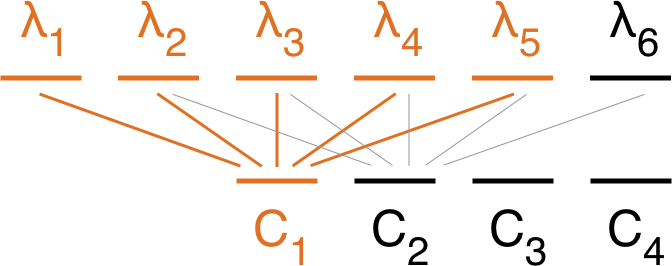
We therefore need to create a sliding window view and then sum over the view's items. The resulting array \(C\) will have \(i-1\) fewer items than \(N\). The count rate relevant for the SNR at \(\lambda_{k}\) is \(C[k - {\rm floor}(i / 2)]\), as illustrated in the image below.
We therefore shift the binset by \({\rm floor}(i / 2)\) to the left. Then \(C\) fulfills the role of \(C(\lambda)\) in the formulae in the SNR section of the simulator physics page.